Decision Trees Learning and Implementation #2

Entropy and Information Gain
Let ‘v’ be the random boolean variable with the following probability distribution:

P(v=0) = 0.2 and P(v=1) = 0.8
Say, v=0 is heads on a coin and v=1 is tails

The surprise S(V=v) of each value ‘v’ is defined as

S(V=v) = -log[P(V=v)]

Which means
– an event with probability 1 gives me ZERO surprise (consider a coin with heads on both sides, and probability of getting heads doesn’t surprise at all)
– an event with probability 0 gives me INFINITE surprise (consider a coin with heads on both sides, and probability of getting tails gives us infinite surprise)

Now that we have individual event surprise, we would be interested in average surprise of all events which introduces the concept of Entropy

What is Entropy? Entropy of ‘v’, denoted as H(v), is defined as the average surprise of describing the result of one trial of ‘v’

Here Sigma(log[P(H=v)]) gives the total surprise and multiplying it with the probability P(H=v) gives the average.

Entropy is also viewed as the measure of uncertainty.

From the graph it is observed that the entropy is maximum at probability=0.5, i.e, when probability is same for both events then the uncertainty is maximum. If you take a fair coin with heads on one side and tails on other side then the

probability P(V=heads)=0.5 and P(V=tails)=0.5
Entropy = -0.5log(0.5)-0.5log(0.5) = 1

In statistics ‘Gene Coefficient’ also generates the same curve as that of entropy.

Now the question is: How this curve helps us to find the best attribute when compared to the error rate? This introduces concept of Information Gain

What is Information Gain or Mutual Information? Consider two dependent random variables A, B. The mutual information between A and B is: the amount of information we learn about B by knowing the value of A.

Mutual Information quantifies how much a feature/attribute ‘x1’ tells about the value of class Y. So now if we look at our previous example

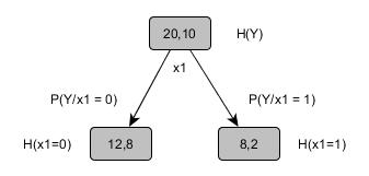
If you notice in previous article the error rate was ZERO before and now we have positive information gain as 0.0304 which is telling us that we are making progress in building the decision tree.

Following the same steps one by one we can build the complete decision tree for the previous shown illustration and it looks sth like this.

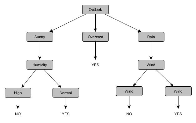
In this graph, if you notice there are only three features (Outlook, Wind and Humidity) considered. We did not consider the remaining feature ‘temperature’ because it is redundant. Even in real time we select only relevant attributes while training the model.

I will dive into the implementation details on some real time data in the next post.