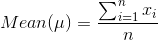
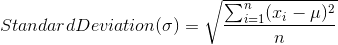
Different Similarity/Distance Measures in Machine Learning

What is the best similarity/distance measure to be used in machine learning models? This depends on various factors. We will see each of them now.

Distance measures for numeric data points

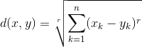
Minkowski Distance: It is a generic distance metric where Manhattan(r=1) or Euclidean(r=2) distance measures are generalizations of it.

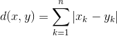
Manhattan Distance: It is the sum of absolute differences between the coordinates. It is also called as Rectilinear Distance, L1-Distance/L1-Norm, Minkowski’s L1 Distance, City Block Distance, Taxi Cab Distance.

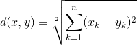
Euclidean Distance: It is the square-root of sum of squares of difference between the coordinates and is given by Pythagorean theorem. Also called as L2 Norm, Ruler Distance. In general, default distance is considered as Euclidean distance.

Use Manhattan or Euclidean distance measures if there are no missing values in the training data set (data is dense)

Cosine Similarity

This measures the cosine of angle between two data points (instances). It is a judgment of orientation rather than magnitude between two instances/vectors with respect to the origin. The cosine of 0degrees is 1 which means the data points are similar and cosine of 90degrees is 0 which means data points are dissimilar (all these angular measures are independent of magnitude).

• Mostly used in high dimensional positive spaces where output is bounded in the range of [0,1].
• Used in Information Retrieval, Text Mining, Recommendation Systems and Classifications. It is also used to measure cohesion between the clusters in Data Mining.
• It is very efficient to evaluate sparse vectors(as only the non-zero dimensions in the space are considered)
• If the attribute vectors are normalized by subtracting the vector means [e.g., Ai – mean(A)], the measure is called centered cosine similarity and is equivalent to the Pearson Correlation Coefficient.

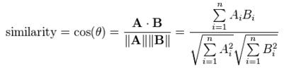
Disadvantage: Cosine similarity is subjective to the domain and application and is not an actual distance metric. For example data points [1,2] and [100,200], are shown similar with cosine similarity, whereas in eucildean distance measure shows they are far away from each other (in a way not similar).

Question #1: If we want to find out closest merchants (like costco, walmart, delta, starbugs, etc) to a given merchant, we would go for cosine similarity because we want merchants in similar domains (i.e, orientation) rather than the magnitude of the feature vector.

Question #2: If we want to find out closest customers to a given customer, we would go for euclidean distance because we want customers who are close in magnitude to the current customer.

Pearson Correlation Coefficient

This is a measure of correlation between two random variables. It ranges between [-1, 1]. 1 is the perfect agreement and -1 is perfect disagreement. We use this when we have grade inflation problem.

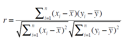
What is grade inflation? It means users are not consistent in giving the ratings. In below example Clara’s 4.75 is same as Robert’s 4 rating. In real time as well some people tend to give extreme ratings and some people never give extreme  ratings and because of this an item (rockband in this case) which is extremely good might get ratings between 4-5 which are all same. And this problem is addressed with pierson coefficient.

Jaccard Similarity

Data points in Jaccard Similarity are sets rather than vectors. Sometimes the equality of certain values does not mean anything and this problem is addressed with Jaccard Similarity.
What is set? Collection of unordered elements {a,b}
What is Cardinality? It counts number of elements in A and is denoted by |A|
Intersection of sets? Elements common in both datasets A and B
Union of Sets? All elements present in both sets.

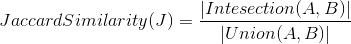
Illustration of iTune songs ordered by number of plays.
Problem Stmt: find similar songs in iTunes

Say, my top track is Moonlight Sonata by Marcus Miller with 25 plays. Chances are that you have played that track zero times. In fact, chances are good that you have not played any of my top tracks. In addition, there are over 15 million tracks in iTunes and I have only four thousand. So the data for a single person is sparse since it has relatively few non-zero attributes (plays of a track). When we compare two people by using the number of plays of the 15 million tracks, mostly they will have shared zeros in common and it doesn’t indicate the similarity between the users. On the other hand, if both users listened to the same song (a value of 1 for each), it is implied that the users have many similarities. In this case, equality of 1 should carry a much higher weight than equality of 0.

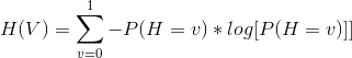
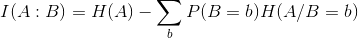
There are other distance measures for sequences (Time Series), network nodes(Sim Rank, Random Walk), population distribution(KL Divergence) which I will be covering in later posts.

REFERENCES
http://www.cse.msu.edu/~pramanik/research/papers/2003Papers/sac04.pdf
https://en.wikipedia.org/wiki/Cosine_similarity
http://dataaspirant.com/2015/04/11/five-most-popular-similarity-measures-implementation-in-python/

Reason for data normalization in ML Models

Standardization/Normalization is a common requirement for majority of algorithms (except like ID3 impl of Trees) which transforms asymmetric training data into symmetric. ML Algorithms behave badly if the training data is not brought on to the same scale because of the noise/outliers or the non-guassian properties of features.

Types of normalization

• Z-transform: This is also called as Standardization.
  • This rescales the features so that they will have the properties of a standard normal distribution with mean=0 and standard_deviation=1.
  • It is useful to standardize attributes for a model that relies on the distribution of attributes such as Gaussian processes.

  

• Normalization: This is also called Min-Max Scaling(based on min max values of the variable).
  • In this data is scaled to a range [0,1].
  • The advantage of this bounded range between 0 and 1 is that it ends up with smaller standard deviations and suppresses the affect of the outliers.
  • We use this method in K-Nearest Neighbors and preparation of coefficients in regression

  

Apart from normalization/standardization techniques, other pre-processing methods to transform data from non-linear to linear can be logarithmic and square root scaling. These are usually performed when the data is characterized by “bursts”, i.e. the data is well grouped in low values, but some portion of it has relatively larger values.

Feature normalization is to make different features to the same. Illustration

Features are Fico_score, Revolving_balance and Num_of_cards. Out of these features, one feature ‘Revolving_Balance’ is in 1000s scale, ‘Fico’ in 100s scale and ‘Num of Cards’ in 10s scale.

Now if we calculate distances between data points, since one of the dimensions have very large values, it overrides other dimensions (you can see above example, the distance contributed by number of cards would completely be nullified by the distance contributed by Revolving_Balance, if the data is not normalized)

The only models that does not care about rescaling of data is when we build the decision trees (like ID3, see the implementation here)

When to use which method? It is hard to say, we have to choose based on some experimentation.

References
https://msdn.microsoft.com/en-us/library/azure/dn905838.aspx
http://scikit-learn.org/stable/modules/generated/sklearn.preprocessing.StandardScaler.html
http://machinelearningmastery.com/rescaling-data-for-machine-learning-in-python-with-scikit-learn/
http://sebastianraschka.com/Articles/2014_about_feature_scaling.html

Importance of data distribution in training machine learning models

A fundamental task in many statistical analyses is to characterize the location and variability of a data set. A further characterization of the data includes data distribution, skewness and kurtosis.

What is Normal Distribution and why is it important in training our data models in Machine learning? The normal distributions are very important class of statistical distributions. All normal distributions are symmetric and have bell-shaped curves with a single peak (aka Gaussian Distribution). Creating a histogram on variable (variable values on Xaxis and its frequency on Yaxis) would get you a normal distribution.

When the distribution is normal then it obeys 68-95-99.7% rule. Which means

• 68% of data points/observations fall within +1*(Standard Deviation) to -1*(Standard Deviation) of mean
• 95% of data points/observations fall within +2*(Standard Deviation) to -2*(Standard Deviation) of mean
• 7% of data points/observations fall within +13*(Standard Deviation) to -3*(Standard Deviation) of mean

If the data distribution is not normal then it can be skewed to the left or right or completely random. Some of these cases are addressed through skewness and kurtosis.

Skewness: The coefficient of Skewness is a measure for the degree of symmetry in the variable distribution. There are different formulae for calculating this skewness coefficient. Karl Pearson gave couple of formula

Kurtosis: Kurtosis is a measure of whether the data are peaked or flat relative to a normal distribution. That is, data sets with high kurtosis tend to have a distinct peak near the mean, decline rather rapidly, and have heavy tails. Data sets with low kurtosis tend to have a flat top near the mean.

Some basics to recollect to go through the distribution (mean, median and std dev)
Mean: It is the sum of all observations divided by number of observations

Median: When all the observations are sorted in the ascending order, the median is exactly the middle value.
– Median is equal to 50^th  percentile.
– If the distribution of the data is Normal, then the median is equal to the arithmetic mean (which also equals Mode).
– The median is not sensitive to extreme values/outliers/noise, and therefore it may be a better measure of central tendency than the arithmetic mean.
Standard Deviation: It gives the measure of the spread of the data. Average of squared differences from the mean is variance and square root of variance is std dev.


References
https://www.mathsisfun.com/data/standard-normal-distribution.html
http://www.itl.nist.gov/div898/handbook/eda/section3/eda35b.htm

ID3 Implementation of Decision Trees

There are different implementations given for Decision Trees. Major ones are

• ID3: Iternative Dichotomizer was the very first implementation of Decision Tree given by Ross Quinlan.
• C4.5: Advanced version of ID3 algorithm addressing the issues in ID3. Some of issues it addressed were
  • Accepts continuous features (along with discrete in ID3)
  • Normalized Information Gain
  • Missing Value Imputation: Handling missing values
  • Pruning: Overfitting problem
  • Applying different weights to the features
• CART: Classification and Regression Trees are similar to C4.5 in many ways except these trees are built on numeric splitting criteria.

We will see the basic implementation of ID3 now and we will extend it from here going further.

INPUTS
Features, training and testing data sets are taken from https://archive.ics.uci.edu/ml/datasets/Hepatitis

FEATURES (sample)

Total: 22
// A listing of the features and their possible values. All features are binary.
age_lte_30 t f
age_betw_31_50 t f
age_gt_50 t f
sex m f

TRAINING DATA (Sample)

Total: 102
trainPatient1 survived   t f f f n y y y y n y y y y y t t t f f f n
trainPatient2 survived   f t f m n y n y y n y y y y y t f t f f t n
trainPatient3 survived   f f t m y y n y y y y y y y y t t t f f f n
trainPatient4 survived   f t f m y n y y y y y y y y y t t t f f f n

TESTING DATA (Sample)

Total: 52
testPatient1 survived    f t f m y y y y y y y y y y y t t f t f f n
testPatient2 survived    f f t m n n y y y n n y y y y t f f f t t y
testPatient3 survived    t f f f y y n n y y n y y y y t f f f t t n
testPatient4 died        f t f m y y n y y y n n y n n t f f t f t y
testPatient5 survived    f f t m n y n n n y n n n y n f f f f t f y

Implementation of the ID3 ALGORITHM

• Load the data: Load the features, training and testing data.
• Build the Decision Tree
• Test the Decision Tree
• Print the constructed Decision Tree

Build the Decision Tree

ALGORITHM
 - Check for the base cases
 - For each attribute, find the Information Gain and choose the attribute 
     with Maximum Info Gain or Minimum Entropy (aka Best Attribute)
 - Create a Decision Node on the best attribute chosen in above step.
 - Recursively run above 3 steps for remaining attributes.

CODE
public DTNode buildDecisionTree(Features features, Instances trainExamples, 
			String[] outputLabels) {

		if(trainExamples.getExamples().size() ==0 || features.getFeatures().size() ==0) {
			return null;
		}

		Map<String, Integer> outputLabelCt = getOutputLabelDistribution(features.getFeatures(), trainExamples.getExamples(), outputLabels);
		int negCt = outputLabelCt.get(outputLabels[0]);
		int posCt = outputLabelCt.get(outputLabels[1]);
		String debug = posCt + "+ve/" + negCt + "-ve";
		
		String outputLabel = outputLabels[1];
		if(posCt > negCt) {
			outputLabel = outputLabels[0];
		}

		if(posCt == 0) {
			DTNode node = new DTNode();
			node.setNodeType(DecisionTreeNodeType.OUTPUT_LEAF_NODE);
			node.setLog(outputLabel+"#ONLYPOS#"+debug);
			node.setOutputLabel(outputLabel);
			return node;
		}

		if(negCt == 0) {
			DTNode node = new DTNode();
			node.setNodeType(DecisionTreeNodeType.OUTPUT_LEAF_NODE);
			node.setLog(outputLabel+"#ONLYNEG#"+debug);
			node.setOutputLabel(outputLabel);
			return node;
		}
		
		Feature bestFeature = getBestFeature(features.getFeatures(), trainExamples.getExamples(), outputLabels, outputLabelCt);
		Features remainingFtrs = getRemainingFtrs(features.getFeatures(), bestFeature);
		//System.out.println("remainingFtrs size "+remainingFtrs.getFeatures().size());

		// build a node based on the best feature
		DTNode root = new DTNode();
		root.setNodeType(DecisionTreeNodeType.FEATURE_NODE);
		root.setLog("#Normal#"+debug);
		root.setFeature(bestFeature);

		// traverse left side and construct
		//System.out.println("traversing left");
		Instances filteredExOnBestFtr = getFilteredExamplesOnBestFtr(trainExamples.getExamples(), bestFeature, bestFeature.getfOptions()[0]);
		root.setLeftNode(buildDecisionTree(remainingFtrs, filteredExOnBestFtr, outputLabels));

		// traverse right side and construct
		//System.out.println("traversing right");
		filteredExOnBestFtr = getFilteredExamplesOnBestFtr(trainExamples.getExamples(), bestFeature, bestFeature.getfOptions()[1]);
		root.setRightNode(buildDecisionTree(remainingFtrs, filteredExOnBestFtr, outputLabels));

		//System.out.println("end");
		// return root of the tree
		return root;
	}

Test the Decision Tree: Tests the decision tree which is built in previous step and prints the accuracy (In our implementation accuracy is around 92%)

Successfully predicted testPatients: 48
Failed example is testPatient5;survived;[f, f, t, m, n, y, n, n, n, y, n, n, n, y, n, f, f, f, f, t, f, y]
Failed example is testPatient19;died;[f, t, f, m, n, n, n, n, y, y, y, y, n, y, y, t, t, f, t, f, t, y]
Failed example is testPatient24;survived;[f, f, t, m, y, y, n, y, y, y, n, n, n, y, n, t, f, t, f, f, t, y]
Failed example is testPatient34;survived;[f, t, f, m, n, y, n, n, n, y, y, y, y, y, y, t, f, f, f, t, f, y]
Number of failed examples: 4, out of total test examples: 52
Accuracy achieved is 92.3076923076923%

OUTPUT Decision Tree

│       ┌── survived#ONLYNEG#1+ve/0-ve
│   ┌── histology#Normal#1+ve/6-ve
│   │   └── died#ONLYPOS#0+ve/6-ve
└── varices#Normal#88+ve/14-ve
    │               ┌── survived#ONLYNEG#4+ve/0-ve
    │           ┌── sex#Normal#9+ve/5-ve
    │           │   │   ┌── died#ONLYPOS#0+ve/4-ve
    │           │   └── sgot_lte_59#Normal#5+ve/5-ve
    │           │       │       ┌── died#ONLYPOS#0+ve/1-ve
    │           │       │   ┌── age_betw_31_50#Normal#1+ve/1-ve
    │           │       │   │   └── survived#ONLYNEG#1+ve/0-ve
    │           │       └── anorexia#Normal#5+ve/1-ve
    │           │           └── survived#ONLYNEG#4+ve/0-ve
    │       ┌── alk_phosphate_lte_127#Normal#35+ve/8-ve
    │       │   │       ┌── survived#ONLYNEG#3+ve/0-ve
    │       │   │   ┌── antivirals#Normal#5+ve/3-ve
    │       │   │   │   │       ┌── survived#ONLYNEG#2+ve/0-ve
    │       │   │   │   │   ┌── sgot_gt_156#Normal#2+ve/1-ve
    │       │   │   │   │   │   └── died#ONLYPOS#0+ve/1-ve
    │       │   │   │   └── liver_big#Normal#2+ve/3-ve
    │       │   │   │       └── died#ONLYPOS#0+ve/2-ve
    │       │   └── spiders#Normal#26+ve/3-ve
    │       │       └── survived#ONLYNEG#21+ve/0-ve
    │   ┌── age_lte_30#Normal#48+ve/8-ve
    │   │   └── survived#ONLYNEG#13+ve/0-ve
    └── fatigue#Normal#87+ve/8-ve
        └── survived#ONLYNEG#39+ve/0-ve

Complete source code can be downloaded at
https://github.com/ntallapa12/decision_tree

References:
https://en.wikipedia.org/wiki/ID3_algorithm
http://www.drdobbs.com/web-development/classifying-text-with-id3-and-c45/184410304
http://stackoverflow.com/questions/9979461/different-decision-tree-algorithms-with-comparison-of-complexity-or-performance

Decision Trees Learning and Implementation #2

Entropy and Information Gain
Let ‘v’ be the random boolean variable with the following probability distribution:

P(v=0) = 0.2 and P(v=1) = 0.8
Say, v=0 is heads on a coin and v=1 is tails

The surprise S(V=v) of each value ‘v’ is defined as

S(V=v) = -log[P(V=v)]

Which means
– an event with probability 1 gives me ZERO surprise (consider a coin with heads on both sides, and probability of getting heads doesn’t surprise at all)
– an event with probability 0 gives me INFINITE surprise (consider a coin with heads on both sides, and probability of getting tails gives us infinite surprise)

Now that we have individual event surprise, we would be interested in average surprise of all events which introduces the concept of Entropy

What is Entropy? Entropy of ‘v’, denoted as H(v), is defined as the average surprise of describing the result of one trial of ‘v’

Here Sigma(log[P(H=v)]) gives the total surprise and multiplying it with the probability P(H=v) gives the average.

Entropy is also viewed as the measure of uncertainty.

From the graph it is observed that the entropy is maximum at probability=0.5, i.e, when probability is same for both events then the uncertainty is maximum. If you take a fair coin with heads on one side and tails on other side then the

probability P(V=heads)=0.5 and P(V=tails)=0.5
Entropy = -0.5log(0.5)-0.5log(0.5) = 1

In statistics ‘Gene Coefficient’ also generates the same curve as that of entropy.

Now the question is: How this curve helps us to find the best attribute when compared to the error rate? This introduces concept of Information Gain

What is Information Gain or Mutual Information? Consider two dependent random variables A, B. The mutual information between A and B is: the amount of information we learn about B by knowing the value of A.

Mutual Information quantifies how much a feature/attribute ‘x1’ tells about the value of class Y. So now if we look at our previous example

If you notice in previous article the error rate was ZERO before and now we have positive information gain as 0.0304 which is telling us that we are making progress in building the decision tree.

Following the same steps one by one we can build the complete decision tree for the previous shown illustration and it looks sth like this.

In this graph, if you notice there are only three features (Outlook, Wind and Humidity) considered. We did not consider the remaining feature ‘temperature’ because it is redundant. Even in real time we select only relevant attributes while training the model.

I will dive into the implementation details on some real time data in the next post.

Decision Trees Learning and Implementation #1

These are most widely used data mining machine learning algorithms for two reasons, one is its fairly easier to understand and implement and other reason is the scalability.

Hypothesis Space and Learning Algorithms of Decision Trees (all these terms are explained in previous article)

• Variable size hypothesis space: Amount of hypothesis space grows with the input data.
• Deterministic: Every training example in Decision Tree is deterministic in nature. (i.e, either positive or negative)
• Parameters: Decision Trees support both continuous and discrete parameters.
• Constructive search algorithms: Tree is built by adding nodes.
• Eager: Learning algorithm of DT is eager in nature.
• Batch Mode.

Some basic concepts of DT hypothesis space
– What is Internal Node? Node where we test the value of one feature [Xj]
– What is a Leaf Node? Leaf nodes makes the class prediction. (if the person has the cancer or not)

Decision Space Decision Boundaries:
– DTs divide feature space into axis parallel rectangles and each rectangle is labeled with one of ‘k’ classes. Consider a simple DTree (on LHS) with two features (X1, X2) with continuous parameters (0-6). The tree is mapped on to a chart on RHS which explains the above definition.

Decision Tree Illustration from Tom Mitchell book (playtennis.data)

From the above data, features (or Attributes) are Outlook, Temperature, Humidity and Wind. With these features we should now build the Decision Tree and the question is which feature comes first in the tree and what other features will follow it?

The order of the features depend on what features you can evaluate fast so that the tree ends quick. If we choose the best attribute every time, then we will be building a great decision tree.

The ideal thing that could happen is to have a feature that perfectly classifies the data (for example spam from non-spam based on some word like , say, ‘viagra’), here the decision tree will be with one feature (say contains_word_viagra) which classifies the data at 100% on one side of node and 0% on other side of the node and we are done.

But in real time it classifies on certain percentages like 60-40, 30-70, 90-10%,etc, (these are also called Error Rates) and we should choose the best feature/attribute as our first node based on best error rate, like 90-10% in above example (because the ideal 100-0% is not possible in real time)

Unfortunately the error rate is not the best factor to choose the attribute because sometimes it does not tell us if we are making any progress while building the decision tree. See the below tree

This tree is not telling us if we made any improvement after splitting on X1, therefore we have to use some better aspect than just the error rate, i.e, To Be Heuristic

A better heuristic from Information Theory is the usage of logarithmic scale which introduces the concept of Entropy and Information Gain. These concepts are explained in the next post.

Essence of Inductive/Supervised Learning

Inductive/Supervised Learning: Given a training example, [x, f(x)], for some unknown function ‘f’, a good approximation of ‘f’ is called Supervised Learning.

Appropriate applications of Supervised Learning

• Situations where humans can perform the task but cannot describe how they do it.
  • x: bitmap picture of hand written characters; f(x): ASCII code of char
• Situation where desired function is changing very frequently.
  • Predictiong stock prices.
• Situation where each user needs customized function.
  • Amazon user recommendations.

Let us take this simple example

#  x1  x2  x3  x4 | y
1  0   0   1   0  | 0  
2  0   1   0   0  | 0  
3  0   0   1   1  | 1  
4  1   0   0   1  | 1  
5  0   1   1   0  | 0  
6  1   1   0   0  | 0  
7  0   1   0   1  | 0  
.
. so on

We have to predict ‘y’ for a given new combination of (x1,x2,x3,x4). Since there are 4 variables, there will be 2^4 states(16) and hence number of functions would become 2^16.

Since the number of functions is double exponential and in real time there will be 1000s of variables, brute force way of finding the function is not possible, therefore we need generalization.

Two views of Machine Learning to generalize

• Removal of remaining uncertainty (suppose we know the unknown function is ‘m of n’, then we would use training examples to infer the function)
• It requires guessing a good, small hypothesis class. We can start with very small class and enlarge it until it contains hypothesis that fits the data.

A framework for hypothesis spaces and learning algorithms

Framework for hypothesis spaces

Key factors to understand the hypothesis space

• Size: Is the hypothesis space fixed in size (like Naïve Bayes) or variable in size (like Decision Trees)
  • Fixed size spaces are easier to understand, but variable size spaces are more useful.
  • Variable size spaces introduce the problem of overfitting.
• Randomness: Is each hypothesis ‘Deterministic’ or ‘Stochastic’? this effects how we evaluate hypothesis.
  • With deterministic hypothesis, the training example is consistent, i.e, correctly predicted OR inconsistent, i.e, incorrectly predicted (ex: spam/non-spam detection)
  • With stochastic hypothesis, the training example is more likely or less likely.
• Parameterization: Is the hypothesis described by set of symbolic (discrete) choices OR continuous parameters?

Framework for Learning Algorithms

Key factors to understand the learning algorithms

• Search Procedure
  • Direct Computation: Solve for the hypothesis directly
  • Local Search: Start with initial hypothesis and make small improvements until local optimum.
  • Constructive Search: We start with empty hypothesis and gradually add structure to it.
• Timing
  • Eager: Analyze training data and construct explicit hypothesis (Decision Trees)
  • Lazy: Store the training data and wait till the testing data is presented and then construct the adhoc hypothesis to classify the test instance (KNN Algo).
• Online vs Batch Learning
  • If the data changes very often (like stock market prediction), we need online learning
  • If the data does not change much overtime (like drug analytics), then we need batch learning. This is more expensive.

Terminology and key issues with Machine Learning

These are some of the terms which are used in machine learning algorithms.

• Training Example: An example of the form [x, f(x)]. Statisticians call it ‘Sample’. It is also called ‘Training Instance’.
• Target Function: This is the true function ‘f’, that we are trying to learn.
• Target Concept: It is a boolean function where
  • f(x) = 1 are called positive instances
  • f(x) = 0 are called negative instances
• Hypothesis: In every algorithm we will try to come up with some hypothesis space which is close to target function ‘f’.
• Hypothesis Space: The space of all hypothesis that can be output by a program. Version Space is a subset of this space.
• Classifier: It’s a discrete valued function.
  • Classifier is what a learner outputs. A learning program is a program where output is also a program.
  • Once we have the classifier we replace the learning algorithm with the classifier.
  • Program vs Output and Learner vs Classifier are same

Some of the notations commonly used in Machine Learning related white papers

Some of the key issues with machine learning algos

• What is a good hypothesis space? Is past data good enough?
• What algorithms fit to what spaces? Different spaces need different algorithms
• How can we optimize the accuracy of future data points? (this is also called as ‘Problem of Overfitting‘)
• How to select the features from the training examples? (this is also called ‘Curse of Dimentionality‘)
• How can we have confidence in results? How much training data is required to find accurate hypothesis (it’s a statistics question)
• Are learning problems computationally intractable? (Is the solution scalable)
• Engineering problem? (how to formulate application problems into ML problems)

Note: Problem of Overfitting and Curse of Dimentionality will be there with most of the real time problems, we will look into each of these problems while studying individual algorithms.

REFERENCES

http://www.cs.waikato.ac.nz/Teaching/COMP317B/Week_1/AlgorithmDesignTechniques.pdf