Decision Trees Learning and Implementation #1
November 9, 2015 Leave a comment
These are most widely used data mining machine learning algorithms for two reasons, one is its fairly easier to understand and implement and other reason is the scalability.
Hypothesis Space and Learning Algorithms of Decision Trees (all these terms are explained in previous article)
- Variable size hypothesis space: Amount of hypothesis space grows with the input data.
- Deterministic: Every training example in Decision Tree is deterministic in nature. (i.e, either positive or negative)
- Parameters: Decision Trees support both continuous and discrete parameters.
- Constructive search algorithms: Tree is built by adding nodes.
- Eager: Learning algorithm of DT is eager in nature.
- Batch Mode.
Some basic concepts of DT hypothesis space
– What is Internal Node? Node where we test the value of one feature [Xj]
– What is a Leaf Node? Leaf nodes makes the class prediction. (if the person has the cancer or not)
Decision Space Decision Boundaries:
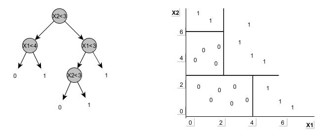
– DTs divide feature space into axis parallel rectangles and each rectangle is labeled with one of ‘k’ classes. Consider a simple DTree (on LHS) with two features (X1, X2) with continuous parameters (0-6). The tree is mapped on to a chart on RHS which explains the above definition.
Decision Tree Illustration from Tom Mitchell book (playtennis.data)
| Day | Outlook | Temperature | Humidity | Wind | Play ball |
| D1 | Sunny | Hot | High | Weak | No |
| D2 | Sunny | Hot | High | Strong | No |
| D3 | Overcast | Hot | High | Weak | Yes |
| D4 | Rain | Mild | High | Weak | Yes |
| D5 | Rain | Cool | Normal | Weak | Yes |
| D6 | Rain | Cool | Normal | Strong | No |
| D7 | Overcast | Cool | Normal | Strong | Yes |
| D8 | Sunny | Mild | High | Weak | No |
| D9 | Sunny | Cool | Normal | Weak | Yes |
| D10 | Rain | Mild | Normal | Weak | Yes |
| D11 | Sunny | Mild | Normal | Strong | Yes |
| D12 | Overcast | Mild | High | Strong | Yes |
| D13 | Overcast | Hot | Normal | Weak | Yes |
| D14 | Rain | Mild | High | Strong | No |
From the above data, features (or Attributes) are Outlook, Temperature, Humidity and Wind. With these features we should now build the Decision Tree and the question is which feature comes first in the tree and what other features will follow it?
The order of the features depend on what features you can evaluate fast so that the tree ends quick. If we choose the best attribute every time, then we will be building a great decision tree.
The ideal thing that could happen is to have a feature that perfectly classifies the data (for example spam from non-spam based on some word like , say, ‘viagra’), here the decision tree will be with one feature (say contains_word_viagra) which classifies the data at 100% on one side of node and 0% on other side of the node and we are done.
But in real time it classifies on certain percentages like 60-40, 30-70, 90-10%,etc, (these are also called Error Rates) and we should choose the best feature/attribute as our first node based on best error rate, like 90-10% in above example (because the ideal 100-0% is not possible in real time)
Unfortunately the error rate is not the best factor to choose the attribute because sometimes it does not tell us if we are making any progress while building the decision tree. See the below tree
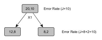
This tree is not telling us if we made any improvement after splitting on X1, therefore we have to use some better aspect than just the error rate, i.e, To Be Heuristic
A better heuristic from Information Theory is the usage of logarithmic scale which introduces the concept of Entropy and Information Gain. These concepts are explained in the next post.

Recent Comments